Blog of Matthew Daws
Ising model and image denoising
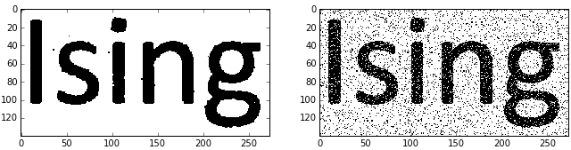
As a final application of MCMC methods, you can't escape the Ising Model, and it's cute application to denoising images (of a text-like nature).
Removing outliers
So, linear regression isn't so exciting. What about removing outliers? I do find this, just a little, magical:
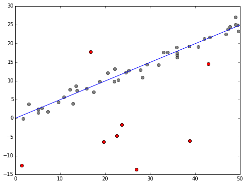
We define a model where a data point \( y_i \) can either be from a normal linear regression model, or just a random (normally distributed) number. We then build into our model indicators \( o_i \in \{0,1\} \) to indicate if this is an outlier or not. Then sample the posterior distribution with an MCMC sampler, integrate out the \(o_i\) and you have your line of best fit. Fix \(i\) and integerate out everything but \(o_i\) and you get an estimate of probability the point is an outlier. The above plot shows those points estimated above 90%.
Rest is in an Ipython notebook on GitHub. This also gave me a chance to play with my own modified Gibbs sampler, which works nicely, if I say so myself.
Read More →Regression from a (simple) Bayesian perspective
How might we tackle simple regression from a Bayesian perpsective? Our model will be that we are given points \( (x_i)_{i=1}^n \) (which we assume we know, at least to a very high accuracy) and dependent points \( y_i^{re} = \alpha + \beta x_i \), but we only observe \( y_i \) where \( y_i = y_i^{re} + e_i \) where the \( e_i \) are our "uncertainties" (I like the line: "if they were errors, we would have corrected them!", see footnote 10 of arXiv:1008.4686) usually modelled as iid \( N(0,\sigma^2) \). The likelihood is then
\[ f(y|\alpha,\beta,\sigma) = \prod (2\pi\sigma^2)^{-1/2} \exp\Big( -\frac{1}{2\sigma^2} (y_i - (\alpha + \beta x_i))^2 \Big) \]
Finding the MLE leads to Least Squares Regression. A simple Bayesian approach would be to stick some prior on $\alpha, \beta, \sigma$, but of course, this raises the question of how to do this!
Anyway, another Ipython notebook which develops some of the basic maths, and then uses emcee and the Triangle Plot to make some simulations and draw some plots of posterior distributions.
Read More →Dabbling in Bayesian Statistics
Bayesian statistics appeals to me both because it seems more "philosophically correct" than frequentist arguments (I have this data, and want to make an inference from it, rather than worrying about data which "might" exist, given other circumstances). Also, Bayesian approaches lead to some interesting computational issues, which are interesting in their own right.
TL;DR: In the process of thinking about MCMC methods in sampling from posterior distributions, I became interested in the choice of prior distributions. Emerging from a lot of reading, you can view my IPython Notebook on finding an "invariant" prior: if you have a natural family of transformations on your "data space" which is reflected in transformations in the parameter space, then I argue there's a natural reason to expect certain invariance in the prior.
For a simple example, consider normally distributed data with known variance. If you translate your data by, say, 5 units, then you would expect your inference about the (unknown) mean to also be exactly translated by 5 units (but to otherwise be the same). This leads to a uniform (improper) prior. I treat the case of unknown mean and variance, which leads to the Jeffreys prior, which is regarded as not so great in the 2 parameter case. Hey ho. This was also a good excuse to learn and play with SymPy.
Read More →Enumerate in C++
One of the fun things about C++11 is that minor changes allow you to write somewhat more expressive (aka Pythonic) code.
A common pattern is to iterate over an array while also knowing the index you are at. Python does this with the enumerate keyword:
for index, x in enumerate(container):
   print("At {} is {}".format(index, x))
In C++ the idiomatic way to do this is perhaps:
std::vector<int> container;
...
for (int i = 0; i < container.size(); ++i) {
   std::cout << "At " << i << " is " << container[i] << "\n";
}
This has its flaws though (and is tedious to type). Using g++, if you have warnings on, -Wall, then you'll see complaint, as the type of container.size() is, typically, of size std::size_t which on my machine is unsigned long long (aka an unsigned 64-bit number). Warnings aside, as int is on my machine a 32-bit unsigned number, we could potentially have problems if the size of container is more than around 2 billion (unlikely, but possible these days).
Jam 2012 Qualification Round
Last one of these for a while. Problem D became an obsession. As ever, links to: Official Contest Analysis and my code on GitHub.
Problem A, Speaking in Tongues: Could be solved with pen and paper, as all the information you need is sneakily in the question.
Read More →Jam 2012 Round 1A
Wrapping up with these... The final problem was rather hard, and in the end was an exercise in profiling... As ever, links to: Official Contest Analysis and my code on GitHub.
Problem A, Password Problem: You have typed A characters of your password, and the probability you typed letter i correctly is \( p_i \), for i=1,...,A. You can press backspace from 0 to A times and type again, or just give up and retype. All your typing will from now on be 100% accurate, and pressing enter counts as a keypress. For each strategy compute the expected number of keypresses needed (if you get the password wrong, you'll have to retype it) and return the lowest expected number of keypresses needed. Your password is B characters in total.
Jam 2015 Round 1C
Urgh, so failure! Some silly (stupid) errors meant my good start of getting problem A out in 16 minutes didn't get me anywhere, as a silly not checking the boundary conditions killed problem B, and not thinking on paper long enough got to problem C. 3 hours and less stress, and it would have been 100/100, but I guess everyone says that about exams. (Of course, given the competition, Round 2 was going to be the end anyway).
As ever, links to: Official Contest Analysis and my code on GitHub.
Problem A, Brattleship: It's in your brother's interest to drag the game out for as long as possible: once he says "hit" we move to a 2nd phase which can only end more quickly.
- So the worst case is when the brat says "miss" until he has no choice but to say hit.
- You want to chop the board up into regions where the ship cannot hit: so strips of width
W-1. So we hit pointsW, 2*W, 3*W, ... - Do each row, and then in the final row, at the final point, brat must say "hit" and we move to a 2nd algorithm of finding the ship.